OOP in R: #1 Intro – Dominik Schulz

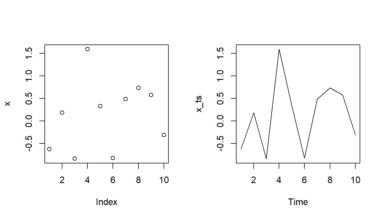
Welcome back to another entry in this blog!

Starting today, I will work on a short series of blog posts on object-oriented programming (OOP) in R. While R itself is a so-called functional programming language, which evolves around defining and chaining functions, it also contains capabilities for OOP. And everyone has come across this neat feature in R, even if without knowing it. OOP in R is for example responsible for why plot() works differently for different types of input, or why we can often just call predict() to generate predictions or forecasts based on a fitted model, (mostly) regardless of the method used for generating the fitted model.

To illustrate the behavior of plot():

set.seed(1)        # starting point for random number generation
x <- rnorm(10)     # just a standard vector
x_ts <- ts(x)      # an object of class "ts"

# Create plots
par(mfrow = c(1, 2), cex = 1)
plot(x)
plot(x_ts)

Figure 1: Example plots for different input objects. Left is a scatter plot, right is a line plot.

When applying plot(x), where x is just a numeric vector, we obtain a scatter plot, where R uses the values of x on the \(y\)-axis. On the contrary, when we apply plot() to an object of class "ts", here to x_ts, which we have created using ts(), the plotting function returns a line plot. Therefore, R can apparently distinguish between different entities and make the same function behave quite differently. During this series, we will investigate, how this behavior arises.

Furthermore, we will consider a very particular example to create our own object class using three different OOP systems in R. In detail, we create a system to better deal with so-called spatial time series. For this purpose, we will use one-minute closing prices of the S&P 500 from September 01, 2026, to September 18, 2026, which are available in my GitHub repository called datasets.

url <- "https://raw.githubusercontent.com/dschulz13/datasets/refs/heads/main/One-minute%20closing%20prices_%5EGSPC_2026-09-01_to_2026-09-20.csv"
dataset <- read.csv(url, check.names = FALSE)
head(dataset, 3)

      Time 2026-09-01 2026-09-02 2026-09-03 2026-09-04 2026-09-08 2026-09-09
1 09:30:00    7629.01    7638.29    7702.06    7736.69    7709.89    7653.67
2 09:31:00    7633.35    7634.67    7701.22    7741.47    7705.91    7651.97
3 09:32:00    7634.28    7640.29    7702.51    7743.00    7704.01    7648.35
  2026-09-10 2026-09-11 2026-09-14 2026-09-15 2026-09-16 2026-09-17 2026-09-18
1    7593.82    7657.91    7597.94    7614.18    7606.13    7641.14    7642.94
2    7592.97    7656.83    7598.48    7604.34    7604.33    7632.16    7647.89
3    7592.08    7661.95    7600.87    7605.97    7603.52    7634.31    7646.34

Especially the plotting of spatial time series can be tedious, as it involves creating 3D figures using libraries such as plotly.

library(plotly)
library(lubridate)
library(dplyr)

dims <- dim(dataset[, -1])

# Matrix with decimal time points
decimal_time <- dataset %>%
  pull(Time) %>%
  hms() %>%
  as.numeric() %>%
  `/`(., 3600) %>%
  rep(dims[[2]]) %>%
  matrix(nrow = dims[[1]], ncol = dims[[2]])

# Matrix with decimal dates
decimal_year <- names(dataset)[-1] %>%
  as.Date() %>%
  decimal_date() %>%
  rep(dims[[1]]) %>%
  matrix(nrow = dims[[1]], ncol = dims[[2]], byrow = TRUE)

# Matrix with closing prices
close <- dataset[, -1] %>%
  unname() %>%
  as.matrix()

# Plot creation
plot_ly(x = decimal_year, y = decimal_time, z = close, type = "surface",
        showscale = FALSE) %>%
  layout(
    scene = list(
      xaxis = list(autorange = "reversed", title = "Decimal year"),
      yaxis = list(autorange = "reversed", title = "Time of day"),
      zaxis = list(title = "Closing price")
    )
  )

Figure 2: A 3D plot of a spatial time series. Readers can also interact with it.

Figure 2 is then a first draft of a plot of a spatial time series that still has a few formatting issues. In a time consuming manner, we need to create matrices for all \(x\), \(y\), and \(z\) coordinates. For better formatting, for example of the decimal year tick labels, we would need to implement further plotly functions. And thus, such a code can easily become quite convoluted. This motivates the development of an object class "spts" (spatial time series), which only contains the observed values and the time points of the two time axes, and to which we may then easily apply predefined standard functions, such as for plotting. This will strongly simplify the workflow in such contexts.

In the next post, we will therefore start implementing such an idea using the S3 system, the simplest OOP system in R. Stay tuned for more!

Best,
Dominik

(Version: September 22, 2026)